
티스토리 뷰
Transformer architectures have become one of the predominant architecture of processing text in NLP. It is typically pre-trained on a large text corpus and then fine-tuned on a task-specific dataset, allowing it to scale effectively to large-scale applications.
Inspired by the success in NLP, many attempts have been made in the vision domain to move away from conventional convolution-based approaches and apply Transformers to images. Prior to this paper, studies combined CNN with attention mechanisms or replaced certain CNN components with attention modules. However, these approaches failed to fully capture global dependencies due to the inherent locality of CNN and high computational cost. Similar to this paper, some study explored using 2 x 2 pixel patches but such method was limited to low-resolution images.
Therefore, this paper suggests dividing images into patches where each patch is considered as a token. By directly applying Transformer architecture to the sequence of image patches, Vision Transformer architecture achieved competitive performance on image classification tasks. From now we will further dive into how Vision Transformer works and the experiment results.
[1] Background
Before discussing the paper, we will first explore the concept of inductive bias, which is one of the key ideas discussed in this work. Inductive bias refers to the prior assumptions a model holds when generalizing from training data. In other words, for a model to learn effectively, it needs some prior knowledge about the underlying structure of the data.

For example, in a fully connected layer, all weights are independent and there is no weight sharing, so the inductive bias is weak. On the other hand, convolutional layers use the same filter across different spatial locations, which introduces an inductive bias of locality. Also, convolution has the property of translation equivariance, which means the features are recognized consistently even when an object moves. Furthermore, recurrent layers share the same function across timesteps, giving them sequential inductive bias.
Compared to convolution, Vision Transformer architecture has much less image-specific inductive bias. This paper shows that a model can learn the structure of images on its own, given that it is trained with a sufficiently large dataset. This will be further explained in the following sections.
[2] Transformer in NLP vs Vision

In NLP, text is first tokenized to be used as an input to the Transformer. These tokens are passed through an embedding layer to generate text embeddings, which are then combined with positional embeddings that encode positional information. The resulting representations serve as the input to the Transformer.
Similarly, in the vision domain, an image is divided into patches, and each patch is linearly projected to obtain its corresponding patch embedding. As in NLP, the patch embeddings are added with positional embeddings to form the final input sequence to the Transformer. However, unlike in NLP where 2D position embeddings are usually used, Vision Transformer used 1D position embeddings. The authors found that 2D-aware positional embeddings did not lead to better performance compared to simpler 1D embeddings, despite being more complex.
In addition, although not shown in the figure above, Vision Transformer uses a special [class] token similar to BERT. This token is added to the patch sequence and serves as an image representation. After passing through the Transformer, the output corresponding to the class token is fed into an MLP head to output the final prediction. The details of this process will be explained in the next section.
[3] Vision Transformer Architecture

The figure above shows the architecture of Vision Transformer presented in the paper. For better understanding, we will break down and explain how each stage is processed.

Let's assume an image of size H × W × C is given.
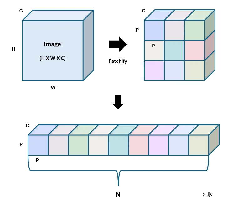
Since we need to convert the image into a sequence of tokens, the image is first divided into small image patches. After patchifying the image, we obtain a total of N patches, each of size P × P × C.

We then convert the N patches obtained from patchifying the image into 1D vectors. By flattening the patches, we obtain a sequence of flattened patch vectors.

As mentioned in the previous section, a special learnable classification token is added to the patch sequence, which serves as the image representation. This token is then passed through a linear projection layer to get the patch embedding.

Finally, the patch embedding obtained earlier is added to 1D positional embedding to form the input to the Transformer.

As illustrated in the figure above, we can summarize the classification process of Vision Transformer. When an image of a dog is given, we first obtain the input to the Transformer as explained earlier. This input is then passed through the Transformer encoder to produce an output sequence. The output corresponding to the classification token is fed into an MLP head to obtain the class label, in this case, "dog". According to the paper, the MLP head consists of two layers with a GELU non-linearity in between.
[4] Fine-tuning with Vision Transformer
Similar to NLP, when applying Transformers to vision tasks, the model is typically pre-trained on a large dataset and then fine-tuned on a smaller downstream task. To do this, the pre-trained prediction head is removed and replaced with a feedforward layer that is initialized to zero.

However, when fine-tuning at a higher resolution than pre-training, the patch size is kept the same, which changes the sequence length. As a result, the positional embeddings learned during pre-training no longer align correctly. For example, if the model was pre-trained at a resolution of 224 × 224, the sequence length would be 196. However, when increasing the resolution to 384 × 384, the sequence length is increased to 576. To solve this issue, the pre-trained position embeddings are interpolated in 2D to match the new sequence length.
[5] Experiments

The paper used three models of different sizes, as described above, to conduct experiments. The models are named based on their size and the input patch size. For example, ViT-L/16 refers to the ViT-Large model using 16 × 16 patches.
5.1 Image Classification Performance
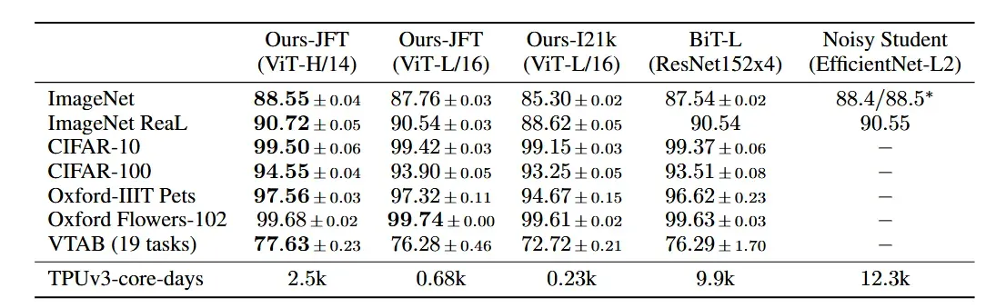
The following results show the performance measured on various benchmarks for image classification. From these results, we can observe three different things.
1) ViT-L/16 [JFT-300M]: Outperforms the CNN-based baseline BiT-L while using fewer computational resources.
2) ViT-H/14 [JFT-300M]: Performance on more challenging tasks have improved by using a larger model than ViT-L/16.
3) ViT-L/16 [ImageNet-21k]: Achieves reasonable results even when pre-trained on the smaller ImageNet dataset instead of JFT.
5.2 Downstream Task Transfer Performance
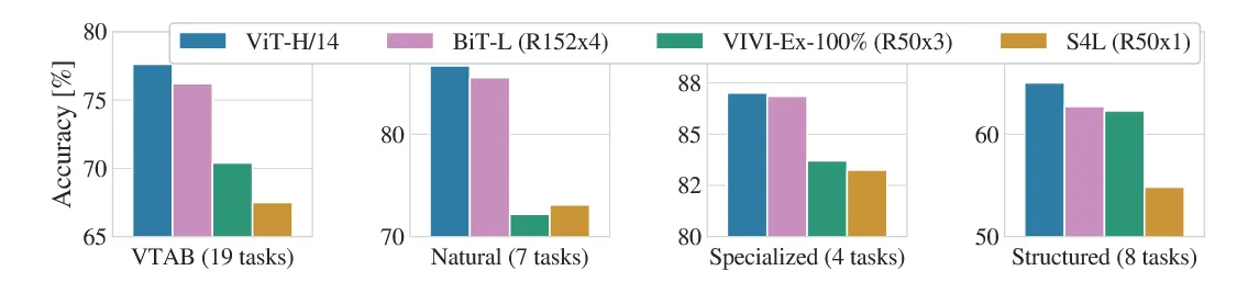
VTAB evaluates low-data transfer performance across 19 different tasks, each using only 1,000 training examples. The tasks are categorized into three groups, natural, specialized, and structured, based on the characteristics of the data. Regardless of the category, Vision Transformer consistently outperforms the CNN baseline across all tasks.
5.3 Pre-training Data Requirements

Vision Transformer shows strong performance when pre-trained on large datasets like JFT-300M, but performance drops noticeably on smaller datasets. Compared to ResNet, Vision Transformer has fewer vision-specific inductive biases, which leads to weaker generalization. To investigate how dataset size affects performance, the paper conducted two experiments.
1) Experiment 1 - Left Figure
- Datasets: ImageNet [1.2M], ImageNet-21K [14M], JFT-300M [~300M]
- Results: When trained on smaller datasets like ImageNet, regularization alone was not enough to improve performance. ViT-Large performed similarly or even worse than ViT-Base. However, when pre-trained on a large dataset, Vision Transformer surpassed the BiT CNN baseline, and we can benefit from using larger models.
2) Experiment 2 - Right Figure
- Datasets: Subsets of JFT-300M / 9M, 30M, 90M, 300M
- Results: When using smaller datasets, CNN-based models with strong inductive biases performed better, while Vision Transformers overfitted more. On the other hand, with larger datasets, Vision Transformer achieved superior performance by learning visual patterns directly from the data despite having weaker inductive biases.
5.4 Scaling Study

A scaling study was conducted to measure transfer accuracy with respect to computational cost. As shown above, when using the same computational budget, Vision Transformers generally outperformed ResNets. This shows that Vision Transformer achieves a better trade-off between training cost and accuracy.
5.5 Inspecting Vision Transformer

1) Patch Embedding - Left Figure
As mentioned earlier in the architecture section, Vision Transformer projects flattened patches into a lower-dimensional space using a linear projection. By observing the 28 principal components of the learned embedding filters, we can confirm that the model successfully learns meaningful low-dimensional representations.
2) Position Embedding - Middle Figure
After the linear projection, Vision Transformer adds positional embeddings. To analyze this, the positional embedding similarities were visualized as above. Results show that nearby patches have similar positional embeddings, and patches in the same row or column show high similarity. This indicates that the model effectively learns positional information.
3) Self-attention Analysis - Right Figure
To understand which regions self-attention focuses on, the average attention distance across different network depths was visualized. In the lower layers, attention distances are broadly distributed, while in the higher layers, they shift toward longer distances. This shows that Vision Transformers integrate global information much earlier than CNNs. Also, at each layer, some heads focus on local patterns while others capture global structures, allowing the model to gradually learn to attend to semantically meaningful regions.
[6] Conclusion
Vision Transformer made a big shift in computer vision by successfully integrating the Transformer architecture to the image domain. It showed that with sufficient data, Transformers can outperform convolutional methods even without convolutional inductive biases. As many modern computer vision studies build upon the Vision Transformer architecture, it is clear that this paper laid the foundation for a new era in computer vision research.
Reference
'논문 리뷰' 카테고리의 다른 글
| [논문 리뷰] Mask R-CNN (1) | 2023.10.13 |
|---|---|
| [논문 리뷰] U-Net: Convolutional Networks for Biomedical Image Segmentation (0) | 2023.09.22 |
| [논문 리뷰] Deep Residual Learning for Image Recognition (0) | 2023.09.14 |